4 November 2026 · Sofia Vallejo · Institute of Electronic Music and Acoustics (IEM), KUG

Modeling the Steiner-Parker filter

I turned a 1970s diode filter into a wave digital model and a free VST3/AU plugin. This is how I did it, how I tested it, and what turned up along the way.

I wanted to model an analog filter that hasn't already been done a hundred times. The Moog ladder, the MS-20 and the TB-303 all have papers and plugins. My first pick was the EDP Wasp, until I found a DAFx 2022 paper that models it already. The Steiner-Parker has a few plugin clones but, as far as I could find, no published circuit model, and its schematic is public. So that's the one.

The plugin is in beta. It runs on macOS as VST3 and AU, and everything is open source.

Download for macOS Code on GitHub

The plugin panel: Frequency and Resonance knobs in red, CV offset and V/oct trim in yellow, Input level and Output in teal, and Response and Quality selectors.

The circuit

Most analog filters use transistors. This one uses a chain of ten 1N4148 diodes with three 1.5 nF capacitors hanging off it. A transistor pair pushes current through the chain, and that current sets the cutoff: more current, higher cutoff.

There are three inputs. Feed the signal in at one point of the network and you get a low-pass, at another a band-pass, at the third a high-pass, all from the same circuit and the same output. On the module that's the Response switch.

I used the schematic from Leonardo Laguna Ruiz's Vult Eurorack build (schematic PDF). It's based on Yves Usson's Yusynth version, which goes back to Nyle Steiner's Synthacon. Every resistor and capacitor value in the model comes from that schematic. This is roughly how the signal moves through it:

The model

I used wave digital filters (WDF). Each capacitor becomes a small WDF element that remembers one value from the last sample. Everything else is nonlinear and tangled together: the diodes, the transistor pair, the op-amps and the resonance feedback. I treat all of that as one block and solve it every sample with Newton's method.

Diodes in series with nothing between them behave like one bigger diode, so the ten diodes collapse into four groups. With the feedback path, the solver ends up with five unknowns per sample, which is small enough to run in real time.

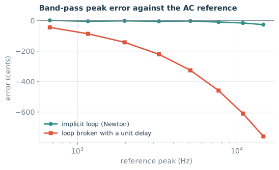
The resonance feedback loops straight back into that block. A common shortcut is to break such a loop with a one-sample delay, but that puts the resonance in the wrong place (more on that below), so I solve the loop as part of the block.

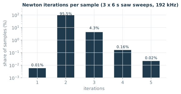
One thing went wrong at first. At high resonance, Newton started jumping back and forth between two answers instead of settling. The fix was the diode step limiting that SPICE uses (pnjlim). After that it settles in two or three steps, even at the top of the resonance range.

The model exists three times, with the same equations in each:

Python (numpy and numba), for the analysis and the plots on this page
C++, the code inside the plugin
JSFX, a version that runs in Reaper without compiling anything

The C++ and JSFX versions match the Python one to within about 1 microvolt.

The build

The plugin is made with JUCE 8 and CMake, so there's no Xcode project to deal with. One script builds a universal binary (Apple silicon and Intel) as VST3, AU and a standalone app, and installs it. A second script packs the beta zip.

xcode-select --install
brew install cmake ninja
cd plugin && ./build_mac.sh

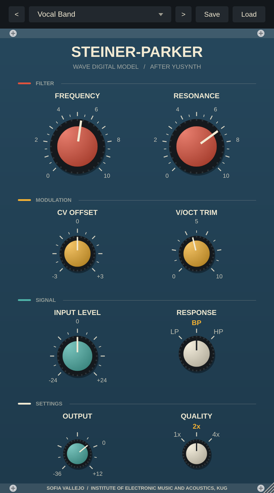
The panel is laid out like a Eurorack module, and the knob colours follow function. Red is the filter (Frequency, Resonance), yellow is modulation (CV offset, V/oct trim), teal is the signal path (Input level, Output), and cream marks the switches. It has 8 factory presets, and you can save and load your own.

Before releasing it I ran Apple's auval and Tracktion's pluginval. Both passed, for the AU and the VST3.

Testing it

I don't have the hardware yet, so I can't compare against a real module. What I can check is whether the simulation actually solves the circuit it's supposed to. For each test I compare the model against something calculated another way.

Frequency response

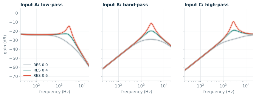
I wrote a second, completely separate analysis that linearizes the circuit and solves it directly in the frequency domain. Then I sent a tiny impulse through the real model, small enough that it behaves linearly, and compared the two.

The feedback loop

This is why I didn't take the one-sample-delay shortcut. With the delay, the resonance peak slides flat as the cutoff goes up. Solved properly, it stays where it should.

Peak error in cents against frequency. The implicit solver stays near zero; the delayed loop falls to minus 760 cents at 14.6 kHz. — **Figure 2.** Where the band-pass peak lands compared to the analysis. Solved properly it stays within 4 cents up to 5 kHz. With the delay it's 44 cents off at 670 Hz and 760 cents off at 14.6 kHz, more than half an octave.

Cutoff range

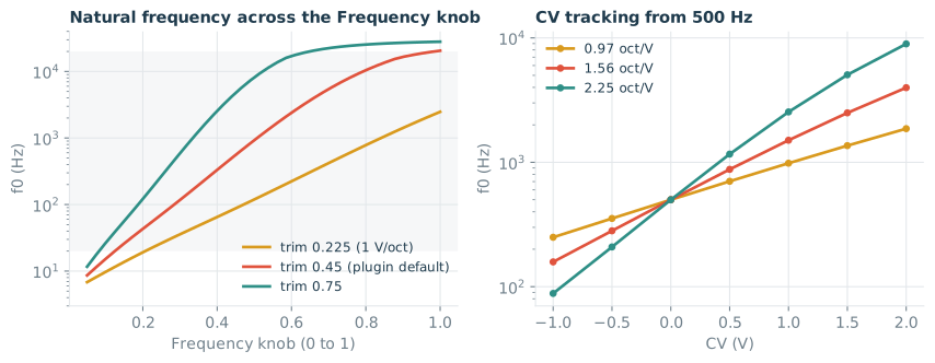
The cutoff is set by a resistor network that adds up the CUT knob, the CV input and a trimmer (T1), which sets how many octaves you get per volt.

You can't have both in this circuit. If you trim it to exactly 1 V/octave, the Frequency knob only covers 10 Hz to 2.5 kHz. That's why my first version sounded so dark. The plugin now defaults to a trim of 0.45, which gives 5 Hz to 20 kHz at about 1.5 octaves per volt.

Left: cutoff frequency against the Frequency knob for three trim settings. Right: frequency against CV, with slopes of 0.97, 1.56 and 2.25 octaves per volt. — **Figure 3.** Left: cutoff across the Frequency knob for three trim settings. The grey band is 20 Hz to 20 kHz. Right: how far the cutoff moves per volt of CV.

Resonance

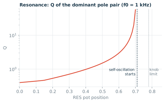
Turning up the resonance pot sends more of the filter's output back into it. At some point the filter starts singing on its own.

Where the dirt comes from

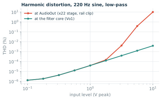
I expected the diodes to give the filter its character. At normal levels they barely do anything. The 47 k input resistor drops the signal about 48 times before it gets to them.

Distortion against input level. At the filter core it stays below 0.01 percent; at the output it rises to about 10 percent at 10 volts. — **Figure 5.** Distortion of a 220 Hz sine through the low-pass. Inside the filter it stays at 0.004% even at 10 V. The output stage, which amplifies 22 times, hits its rails and reaches about 10%. So the plugin's Drive knob mostly drives that output stage, and the resonance once it's high.

Self-oscillation pitch

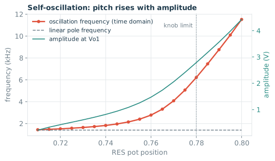
When the filter self-oscillates, its pitch goes up as it gets louder. The linear analysis says it should sit near 1 kHz. In the time-domain model it starts at 1.4 kHz and reaches 6.2 kHz at the end of the knob.

Oscillation frequency rising from 1.4 kilohertz at onset to 6.2 kilohertz at the knob limit while the linear pole frequency stays near 1 kilohertz; amplitude grows alongside. — **Figure 6.** Self-oscillation in the plugin's C++ model at 192 kHz, cutoff set to 1 kHz. It isn't a numerical problem, because it comes out the same at 4x and 16x oversampling. It could still come from my simplifications (an ideal transistor pair, no diode capacitance), so I want to measure a real module before calling it a feature.

How hard the solver works

Bar chart: 95 percent of samples need 2 Newton iterations, about 4 percent need 3, under 0.2 percent need 4 or 5. — **Figure 7.** Newton steps per sample over 3.5 million samples: saw sweeps through all three inputs. It averages 2.05 steps and never goes above 5. In stereo with 2x oversampling, the plugin runs about 7 times faster than real time on one CPU core.

Everything else

Check	Result
Plugin C++ against the Python model	max 0.8 µV	PASS
JSFX against the Python model	max 1.4 µV	PASS
Apple `auval`, 11 to 192 kHz	all tests	PASS
`pluginval` strictness 5, VST3 and AU	all tests	PASS
Stress test: every mode, +24 dB drive, full resonance, fast cutoff jumps	no NaNs	PASS

Listen

A 55 Hz sawtooth at Eurorack level (5 V), with the cutoff sweeping slowly up and back down.

Low-passinput A, resonance 0.55

Band-passinput B, resonance 0.55

High-passinput C, resonance 0.55

Low-pass, almost singinginput A, resonance 0.74

What's missing

A real module to compare against. If you have a Yusynth or Vult build and can record it, please write to me.
Some parts are idealized. The transistor pair is ideal, the diodes have no capacitance, and the op-amps are perfect amplifiers with a soft clip at the rails.
The top of the resonance pot is left out. Above about 0.8, the model starts oscillating at 15 to 28 kHz and the solver struggles. I think that comes from the simplifications above, so it stays out until I can check it.
No all-pass setting. The Yusynth panel has an AP position. The Vult build doesn't, and I'm not adding it without seeing the real wiring.
Mac only, and not notarized. macOS needs one Terminal command after installing (below). Windows and Linux builds should work from the same code, but I haven't released them yet.

Try the beta

Download the zip and unzip it.
Copy Steiner-Parker Filter.vst3 into ~/Library/Audio/Plug-Ins/VST3/ and Steiner-Parker Filter.component into ~/Library/Audio/Plug-Ins/Components/. In Finder, use Go > Go to Folder and paste the path.
Open Terminal and paste these two lines. They only remove the "downloaded from the internet" flag from those two files.

xattr -dr com.apple.quarantine ~/Library/Audio/Plug-Ins/VST3/"Steiner-Parker Filter.vst3"
xattr -dr com.apple.quarantine ~/Library/Audio/Plug-Ins/Components/"Steiner-Parker Filter.component"

Rescan plugins in your DAW and look for Steiner-Parker Filter by Sofia Vallejo. AU plugins show up after restarting the DAW.

Found a bug, or something sounds off? Open an issue and tell me your DAW, sample rate and settings.

Credits

The circuit is by Nyle Steiner (the Synthacon), Yves Usson (Yusynth) and Leonardo Laguna Ruiz (Vult), whose schematic values the model uses. The plugin only models how the circuit behaves; it doesn't include their drawings or PCB files. It's built with JUCE 8, and the VST3 SDK is by Steinberg. The code is open source under the GNU AGPL v3.